Lesson 7: Logistic Regression for Public Health

Modeling Binary Health Outcomes

Learning Objectives

By the end of this lesson, you will be able to:

  • Explain when logistic regression is appropriate
  • Interpret odds and probabilities in health research
  • Fit a logistic regression model in R
  • Interpret odds ratios in public health language
  • Generate predicted probabilities
  • Communicate findings responsibly

Assigned Readings

  • OpenIntro Biostatistics, Chapter 8
  • Statistical Inference via Data Science, Chapter 6

1. When Do We Use Logistic Regression?

Linear regression is used when:

  • Outcome is continuous (BMI, blood pressure, cholesterol)

Logistic regression is used when:

  • Outcome is binary
    • Hypertension: Yes / No
    • Diabetes: Yes / No
    • Smoker: Yes / No
    • Fair/Poor health: Yes / No

Logistic regression models:

[ log() = _0 + _1X ]

Where:

  • (p) = probability of the outcome
  • (p/(1-p)) = odds

2. Load NHANES Data

Loading Libraries

library(tidyverse)
Warning: package 'dplyr' was built under R version 4.5.1
── Attaching core tidyverse packages ──────────────────────── tidyverse 2.0.0 ──
✔ dplyr     1.2.0     ✔ readr     2.1.5
✔ forcats   1.0.0     ✔ stringr   1.5.1
✔ ggplot2   3.5.2     ✔ tibble    3.2.1
✔ lubridate 1.9.4     ✔ tidyr     1.3.1
✔ purrr     1.0.4     
── Conflicts ────────────────────────────────────────── tidyverse_conflicts() ──
✖ dplyr::filter() masks stats::filter()
✖ dplyr::lag()    masks stats::lag()
ℹ Use the conflicted package (<http://conflicted.r-lib.org/>) to force all conflicts to become errors
library(NHANES)

Loading the Dataset & Creating a Subsect

data(NHANES)

df <- NHANES %>%
  filter(!is.na(BMI), !is.na(Gender), !is.na(Age)) %>%
  mutate(
    high_bmi = ifelse(BMI >= 30, 1, 0)
  )

3. Fit Logistic Regression Model

Our example research question: Is obesity associated with age?

model <- glm(high_bmi ~ Age, 
             data = df, 
             family = binomial)

summary(model)

Call:
glm(formula = high_bmi ~ Age, family = binomial, data = df)

Coefficients:
             Estimate Std. Error z value Pr(>|z|)    
(Intercept) -1.865791   0.051335  -36.34   <2e-16 ***
Age          0.023872   0.001084   22.01   <2e-16 ***
---
Signif. codes:  0 '***' 0.001 '**' 0.01 '*' 0.05 '.' 0.1 ' ' 1

(Dispersion parameter for binomial family taken to be 1)

    Null deviance: 11552  on 9633  degrees of freedom
Residual deviance: 11040  on 9632  degrees of freedom
AIC: 11044

Number of Fisher Scoring iterations: 4

What Is Happening Here?

  • glm() fits a generalized linear model.
  • family = binomial specifies a binary outcome.
  • The model estimates log-odds, not probabilities.

The coefficient for Age is on the log-odds scale.

It must be transformed before interpretation.

4. Convert Coefficients to Odds Ratios

exp(coef(model))
(Intercept)         Age 
  0.1547737   1.0241594 

Interpretation:

Each additional year of age is associated with a 2% increase in the odds of obesity.

Interpretation Rules

  • OR = 1 → No association
  • OR > 1 → Increased odds
  • OR < 1 → Decreased odds

Examples:

  • OR = 1.25 → 25% higher odds
  • OR = 0.80 → 20% lower odds

5. Confidence Intervals for Odds Ratios

exp(confint(model))
Waiting for profiling to be done...
                2.5 %    97.5 %
(Intercept) 0.1398656 0.1710458
Age         1.0219920 1.0263459

Interpretation framework:

Each one-year increase in age was associated with a ___-fold increase in odds of obesity (95% CI: lower to upper).

How to Interpret Confidence Intervals

  • If the CI includes 1 → not statistically significant
  • If the CI does not include 1 → statistically significant
  • CIs communicate magnitude and uncertainty

In public health research, effect size and uncertainty matter more than p-values alone.

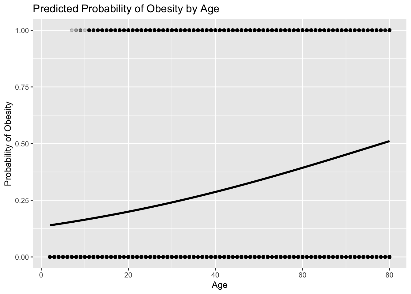
6. Predicted Probabilities

Odds ratios can be abstract.

Public health audiences often understand probabilities better.

new_ages <- tibble(Age = c(20, 40, 60))

predicted <- predict(model, new_ages, type = "response")

cbind(new_ages, predicted_probability = predicted)
  Age predicted_probability
1  20             0.1996715
2  40             0.2868146
3  60             0.3932998

type = "response" converts log-odds into probabilities.

Interpretation Example

  • If predicted probability at age 20 = 0.18 → 18% probability of obesity
  • If predicted probability at age 60 = 0.34 → 34% probability of obesity

Notice

  • The increase is nonlinear.
  • Predicted values stay between 0 and 1.
  • Logistic regression produces an S-shaped curve.

7. Visualizing Logistic Model

age_grid <- tibble(Age = seq(min(df$Age), max(df$Age), length.out = 200))

age_grid$prob <- predict(model, age_grid, type = "response")

ggplot(df, 
       aes(
         x = Age, 
         y = high_bmi
         )) +
  geom_point(alpha = 0.2) +
  geom_line(data = age_grid, 
            aes(
              Age, 
              prob), 
            linewidth = 1.2) +
  labs(y = "Probability of Obesity",
       title = "Predicted Probability of Obesity by Age")

What to observe:

  • Points are binary (0 or 1).
  • The curve is smooth.
  • Probability increases gradually.
  • Predictions remain within logical bounds.

Linear regression could predict probabilities below 0 or above 1. Logistic regression avoids that issue.

8. Odds vs. Probability (Concept Clarification)

People often confuse odds and probability.

Probability is the chance that the event occurs. The range is 0 to 1.

Odds are the probability of something divided by 1 minus that probability.

So, if the probability of something happening is 0.20, the the odds are (.20)/(1-.20) = (.20)/(.80) = .25.

Odds can exceed 1, probability cannot.

Why Logistic Regression Uses Odds

  • Odds range from 0 to infinity.
  • Log(odds) ranges from negative infinity to positive infinity.
  • This makes the model mathematically stable.

Important:

  • Odds ratio ≠ risk ratio.
  • An OR of 2 does not mean “twice as likely” unless the outcome is rare.

9. Public Health Interpretation

Avoid:

  • “Age causes obesity.”
  • “Risk doubles.”

Use:

  • “Age was associated with higher odds of obesity.”
  • “After adjustment, age remained independently associated with obesity.”

Limitations to Consider

  • Cross-sectional data cannot establish causality.
  • Measurement error may bias results.
  • Residual confounding may remain.
  • Survey design limitations may affect inference.

Logistic Regression Assumptions (Introductory)

  • Independent observations
  • Correct link function
  • No severe multicollinearity
  • Adequate sample size