Lesson 11: Hypothesis Testing

Simulation-First Thinking, P-values, and Biomedical Interpretation

Overview

Hypothesis testing allows us to evaluate whether observed patterns in data are likely due to chance or reflect a real underlying relationship.

In this lesson, we take a simulation-first approach to hypothesis testing, emphasizing intuition, interpretation, and real-world biomedical framing rather than memorizing formulas.

Learning Objectives

By the end of this lesson, students will be able to:

Explain the logic of hypothesis testing using simulation
Define null and alternative hypotheses in public health contexts
Interpret p-values as measures of evidence strength
Avoid common misinterpretations of p-values
Apply hypothesis testing to real-world biomedical questions
Connect hypothesis testing to regression inference

Assigned Readings

OpenIntro Biostatistics, Chapter 5
Statistical Inference via Data Science, Chapter 10: Inference for Regression

What Is Hypothesis Testing?

Hypothesis testing is a framework used to evaluate whether observed data are consistent with a specific claim about a population.

We compare:

what we observed in our data
what we would expect under a null hypothesis

Null and Alternative Hypotheses

The null hypothesis (H₀) represents no effect or no association.

The alternative hypothesis (H₁ or Hₐ) represents a meaningful effect or association.

Example (Public Health)

H₀: There is no difference in screening rates between groups
Hₐ: There is a difference in screening rates between groups

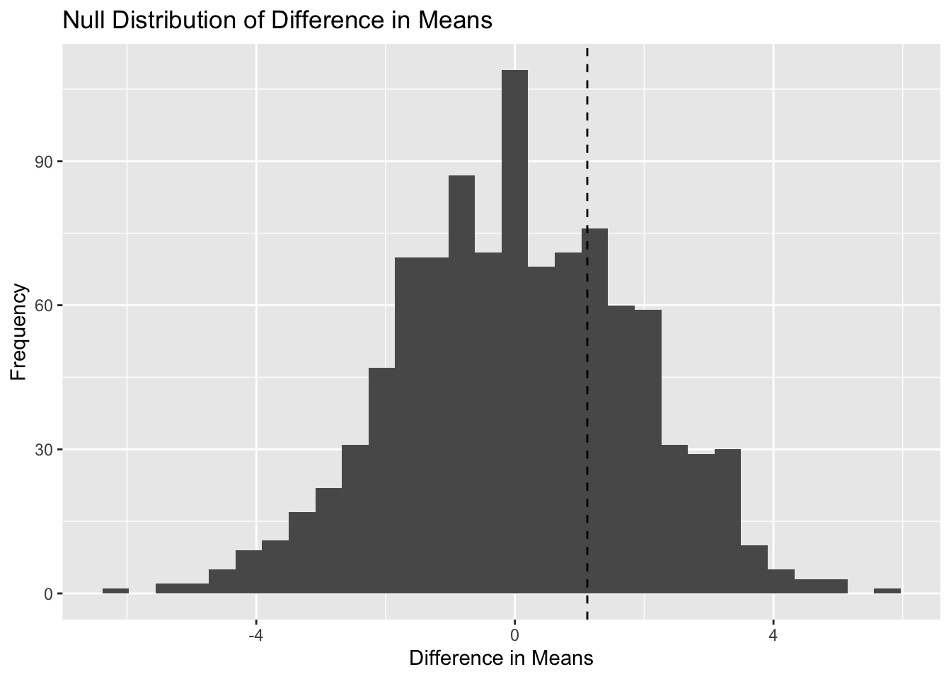
Simulation-First Thinking

Instead of jumping straight to formulas, we ask:

What would our data look like if the null hypothesis were true?

We then simulate many datasets under the null and compare our observed statistic to that distribution.

Example: Simulating a Null Distribution

library(tidyverse)

Warning: package 'dplyr' was built under R version 4.5.1

── Attaching core tidyverse packages ──────────────────────── tidyverse 2.0.0 ──
✔ dplyr     1.2.0     ✔ readr     2.1.5
✔ forcats   1.0.0     ✔ stringr   1.5.1
✔ ggplot2   3.5.2     ✔ tibble    3.2.1
✔ lubridate 1.9.4     ✔ tidyr     1.3.1
✔ purrr     1.0.4     
── Conflicts ────────────────────────────────────────── tidyverse_conflicts() ──
✖ dplyr::filter() masks stats::filter()
✖ dplyr::lag()    masks stats::lag()
ℹ Use the conflicted package (<http://conflicted.r-lib.org/>) to force all conflicts to become errors

set.seed(123)

# Create two groups with no real difference
group <- rep(c("A", "B"), each = 50)
outcome <- rnorm(100, mean = 50, sd = 10)

df <- tibble(group, outcome)

# Observed difference in means
obs_diff <- df |>
  group_by(group) |>
  summarise(mean_val = mean(outcome)) |>
  summarise(diff = diff(mean_val)) |>
  pull(diff)

obs_diff

[1] 1.120047

Permutation Test (Simulation)

set.seed(123)

null_dist <- replicate(1000, {
  shuffled <- df |>
    mutate(group = sample(group))

  shuffled |>
    group_by(group) |>
    summarise(mean_val = mean(outcome)) |>
    summarise(diff = diff(mean_val)) |>
    pull(diff)
})

null_df <- tibble(diff = null_dist)

Visualizing the Null Distribution

ggplot(null_df, aes(x = diff)) +
  geom_histogram(bins = 30) +
  geom_vline(xintercept = obs_diff, linetype = "dashed") +
  labs(
    title = "Null Distribution of Difference in Means",
    x = "Difference in Means",
    y = "Frequency"
  )

Interpreting the Simulation

The histogram shows what differences we would expect if there were no real effect
The dashed line shows our observed result
We assess how extreme our observed value is relative to the null distribution

What Is a P-value?

The p-value is the probability of observing a result as extreme (or more extreme) than what we observed, assuming the null hypothesis is true.

Calculating the P-value

p_value <- mean(abs(null_df$diff) >= abs(obs_diff))
p_value

[1] 0.56

Interpreting the P-value

Small p-value → strong evidence against the null
Large p-value → weak evidence against the null

P-values as Evidence Strength

P-value	Interpretation
< 0.01	Very strong evidence
0.01–0.05	Strong evidence
0.05–0.10	Moderate evidence
> 0.10	Weak evidence

What P-values Do NOT Mean

❌ The probability that the null hypothesis is true
❌ The probability that the results are due to chance alone
❌ The size or importance of an effect

Decision-Making Framework

We often compare the p-value to a significance level (α), commonly 0.05.

If p-value < 0.05 → reject H₀
If p-value ≥ 0.05 → fail to reject H₀

Biomedical Framing

In public health and medicine, hypothesis testing answers questions like:

Does a treatment improve outcomes?
Is an exposure associated with disease?
Do disparities persist between populations?

Example Interpretation

The intervention group had lower blood pressure than the control group (p = 0.03).

Interpretation:

There is evidence of a difference
The observed result is unlikely under the null
The effect may be meaningful, but magnitude should also be considered

Hypothesis Testing in Regression

Hypothesis testing is also used in regression models.

Example:

H₀: β₁ = 0 (no association between predictor and outcome)
Hₐ: β₁ ≠ 0

Example in R

model <- lm(outcome ~ group, data = df)
summary(model)


Call:
lm(formula = outcome ~ group, data = df)

Residuals:
     Min       1Q   Median       3Q      Max 
-24.5558  -5.9140  -0.5798   6.5742  21.3455 

Coefficients:
            Estimate Std. Error t value Pr(>|t|)    
(Intercept)   50.344      1.295  38.875   <2e-16 ***
groupB         1.120      1.831   0.612    0.542    
---
Signif. codes:  0 '***' 0.001 '**' 0.01 '*' 0.05 '.' 0.1 ' ' 1

Residual standard error: 9.157 on 98 degrees of freedom
Multiple R-squared:  0.003802,  Adjusted R-squared:  -0.006363 
F-statistic: 0.374 on 1 and 98 DF,  p-value: 0.5422

Interpreting Regression Output

The coefficient represents the estimated effect
The p-value tests whether that effect is different from zero
Confidence intervals provide a range of plausible values

Connecting to Confidence Intervals

If CI excludes 0 (or 1 for ratios) → statistically significant
If CI includes 0 → not statistically significant

Key Terms

Term	Definition
Null Hypothesis	No effect or association
Alternative Hypothesis	Presence of effect
Test Statistic	Measure of observed effect
Null Distribution	Distribution under H₀
P-value	Probability of extreme result under H₀
Significance Level	Threshold for decision-making

Practice Activity

Simulate a null distribution
Compute an observed statistic
Calculate a p-value
Interpret the result in plain language
Decide whether to reject the null

Reflection Questions

Why do we simulate under the null hypothesis?
What does a small p-value tell us?
Why is statistical significance not the same as practical importance?
How does this apply to real public health decisions?

Common Mistakes to Avoid

Treating p-value as probability the null is true
Ignoring effect size
Over-relying on 0.05 cutoff
Confusing statistical and clinical significance

Conclusion

Hypothesis testing provides a structured way to evaluate evidence.

A simulation-first approach helps build intuition by showing what results look like under the null hypothesis.

P-values quantify evidence strength, but must be interpreted carefully and alongside effect sizes and confidence intervals.

Looking Ahead

Next lesson:

Multiple testing
Type I and Type II errors
Power and sample size