Lesson 9: Introduction to Statistical Inference

Sampling Variability, Standard Error, Simulation Intuition, and Uncertainty

Overview

Statistical inference helps us use data from a sample to learn about a larger population. In public health, we often do not have access to an entire population, so we rely on sample data to estimate population values and quantify uncertainty.

In this lesson, we will introduce the foundational ideas behind statistical inference, including sampling variability, standard error, simulation intuition, and the connection between observed data and uncertainty.

Learning Objectives

By the end of this lesson, students will be able to:

• Define statistical inference in the context of public health research
• Explain sampling variability and why sample estimates differ
• Define and interpret the standard error
• Use simulation to build intuition about uncertainty
• Explain how confidence intervals connect data to uncertainty
• Interpret results from estimation procedures in plain language

Assigned Readings

• OpenIntro Biostatistics, Chapter 3
• Statistical Inference via Data Science, Chapter 8: Estimation, Confidence Intervals, and Bootstrapping

What Is Statistical Inference?

Statistical inference is the process of using sample data to draw conclusions about a population.

For example, researchers may want to estimate:

• the average body mass index in a community
• the proportion of adults who are up to date on cancer screening
• the difference in blood pressure between two treatment groups

Because these values are usually unknown for the full population, we use sample statistics to estimate them.

From Sample to Population

A population is the full group we want to understand.

A sample is the subset of that population that we actually observe.

A parameter is a numerical summary of the population, such as a population mean or population proportion.

A statistic is a numerical summary calculated from the sample, such as a sample mean or sample proportion.

Statistical inference uses sample statistics to estimate unknown population parameters.

Sampling Variability

One of the most important ideas in inference is sampling variability.

If we take many different random samples from the same population, the sample results will not be exactly the same each time. This happens because each sample contains slightly different observations.

That natural variation from sample to sample is called sampling variability.

Why Sampling Variability Matters

Sampling variability explains why we should not expect one sample statistic to equal the true population value exactly.

It also explains why we need tools like:

• standard errors
• confidence intervals
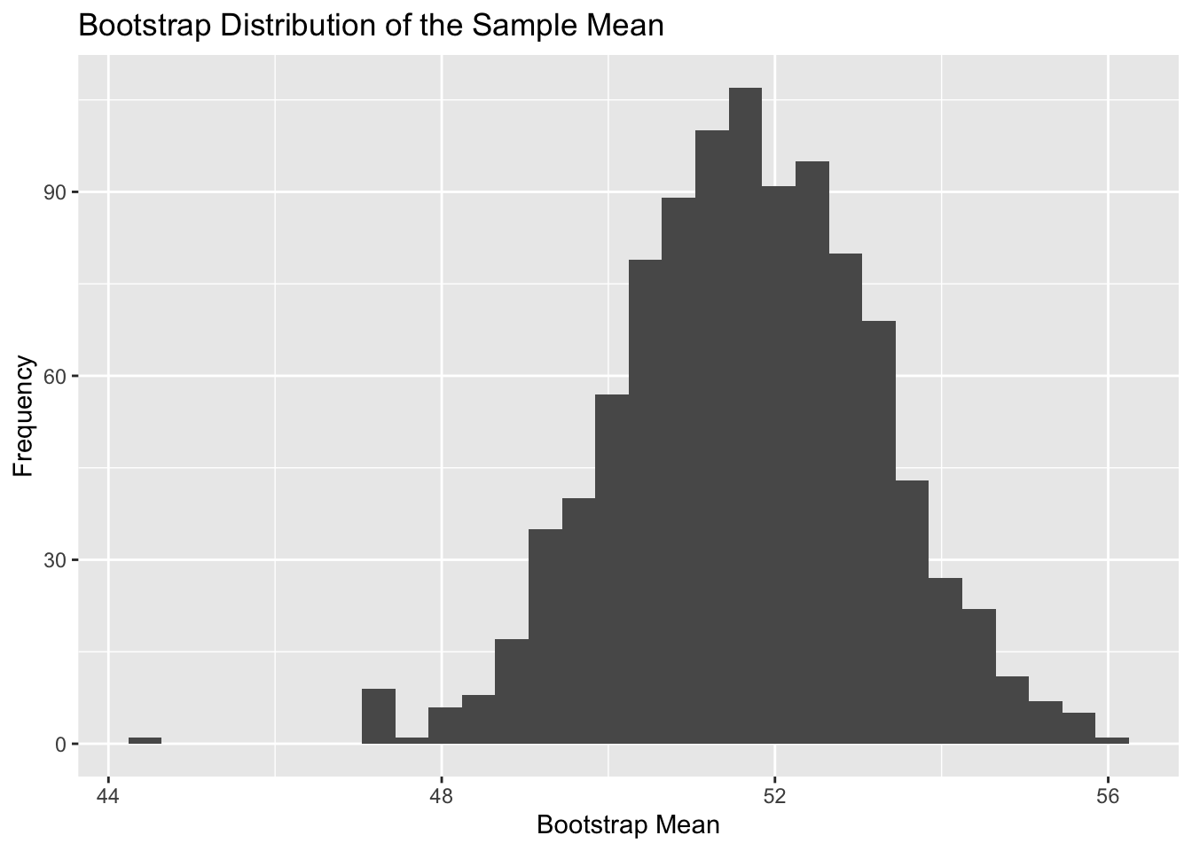
• bootstrap distributions
• hypothesis tests

These tools help us measure and communicate uncertainty.

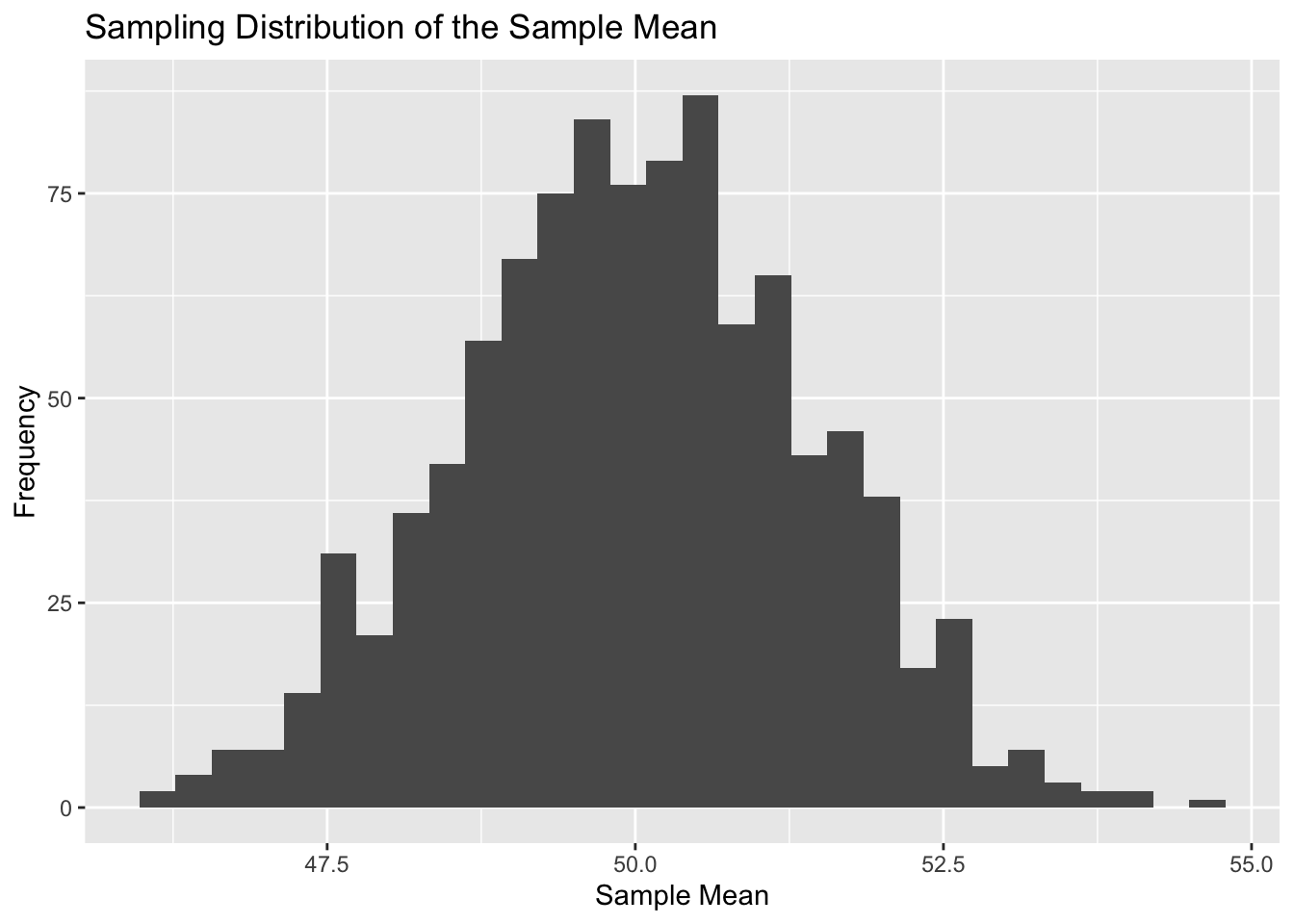
Example: Simulating a Population

In the example below, we create a population and repeatedly draw samples from it. Then we compute the sample mean for each sample.

library(tidyverse)

Warning: package 'dplyr' was built under R version 4.5.1

── Attaching core tidyverse packages ──────────────────────── tidyverse 2.0.0 ──
✔ dplyr     1.2.0     ✔ readr     2.1.5
✔ forcats   1.0.0     ✔ stringr   1.5.1
✔ ggplot2   3.5.2     ✔ tibble    3.2.1
✔ lubridate 1.9.4     ✔ tidyr     1.3.1
✔ purrr     1.0.4     
── Conflicts ────────────────────────────────────────── tidyverse_conflicts() ──
✖ dplyr::filter() masks stats::filter()
✖ dplyr::lag()    masks stats::lag()
ℹ Use the conflicted package (<http://conflicted.r-lib.org/>) to force all conflicts to become errors

set.seed(123)

population <- tibble(
  value = rnorm(10000, mean = 50, sd = 10)
)

head(population)

# A tibble: 6 × 1
  value
  <dbl>
1  44.4
2  47.7
3  65.6
4  50.7
5  51.3
6  67.2

Repeated Sampling

Now we take many random samples of size 50 and calculate the mean for each sample.

set.seed(123)

sample_means <- replicate(1000, {
  population |>
    slice_sample(n = 50) |>
    summarise(mean_value = mean(value)) |>
    pull(mean_value)
})

sample_means_df <- tibble(sample_mean = sample_means)

head(sample_means_df)

# A tibble: 6 × 1
  sample_mean
        <dbl>
1        49.9
2        47.5
3        50.4
4        51.0
5        50.1
6        50.4

Visualizing Sampling Variability

ggplot(sample_means_df, aes(x = sample_mean)) +
  geom_histogram(bins = 30) +
  labs(
    title = "Sampling Distribution of the Sample Mean",
    x = "Sample Mean",
    y = "Frequency"
  )

Interpreting the Plot

This histogram shows the distribution of sample means across many repeated samples.

Notice:

• the sample means are not all identical
• most sample means cluster around the true population mean
• some sample means are a little higher or lower just by chance

This is sampling variability in action.

The Standard Error

The standard error tells us how much a sample statistic tends to vary from sample to sample.

For a sample mean, the standard error is often written as:

\[ SE = \frac{s}{\sqrt{n}} \]

where:

• ( s ) is the sample standard deviation
• ( n ) is the sample size

Interpreting the Standard Error

A smaller standard error means the estimate is more precise.

A larger standard error means the estimate is less precise.

In general:

• larger samples produce smaller standard errors
• more variability in the data produces larger standard errors

Calculate a Standard Error

set.seed(456)

sample_data <- population |>
  slice_sample(n = 50)

sample_mean <- mean(sample_data$value)
sample_sd <- sd(sample_data$value)
sample_n <- nrow(sample_data)
sample_se <- sample_sd / sqrt(sample_n)

sample_mean

[1] 51.61875

sample_sd

[1] 10.79668

sample_n

[1] 50

sample_se

[1] 1.526882

Plain-Language Interpretation

The sample mean is our estimate of the population mean.

The standard error tells us how much we would expect that estimate to change across repeated random samples of the same size.

How Sample Size Affects Standard Error

Let us compare standard errors for different sample sizes.

set.seed(789)

get_se <- function(n) {
  samp <- population |>
    slice_sample(n = n)
  sd(samp$value) / sqrt(n)
}

se_50 <- get_se(50)
se_200 <- get_se(200)
se_500 <- get_se(500)

tibble(
  sample_size = c(50, 200, 500),
  standard_error = c(se_50, se_200, se_500)
)

# A tibble: 3 × 2
  sample_size standard_error
        <dbl>          <dbl>
1          50          1.29 
2         200          0.716
3         500          0.460

Interpretation of Sample Size Comparison

As the sample size increases, the standard error usually gets smaller.

This means larger samples tend to produce more stable and precise estimates.

Simulation Intuition

Sometimes formulas can feel abstract. Simulation helps us build intuition by letting us see uncertainty directly.

Instead of only calculating a standard error with a formula, we can simulate many samples and watch the estimate vary.

This helps students understand that uncertainty is not a flaw in the data. It is a natural part of working with samples.

Bootstrap Intuition

Bootstrapping is a simulation-based method for estimating uncertainty.

The basic idea is:

1. Start with your observed sample.
2. Resample from that sample with replacement many times.
3. Calculate the statistic of interest for each resample.
4. Use the resulting distribution to understand variability and build confidence intervals.

Bootstrap Example

library(infer)

Warning: package 'infer' was built under R version 4.5.1

set.seed(101)

boot_dist <- sample_data |>
  specify(response = value) |>
  generate(reps = 1000, type = "bootstrap") |>
  calculate(stat = "mean")

head(boot_dist)

Response: value (numeric)
# A tibble: 6 × 2
  replicate  stat
      <int> <dbl>
1         1  55.3
2         2  51.9
3         3  49.3
4         4  50.9
5         5  50.2
6         6  50.2

Visualizing the Bootstrap Distribution

ggplot(boot_dist, aes(x = stat)) +
  geom_histogram(bins = 30) +
  labs(
    title = "Bootstrap Distribution of the Sample Mean",
    x = "Bootstrap Mean",
    y = "Frequency"
  )

What the Bootstrap Distribution Shows

The bootstrap distribution shows the range of values we might reasonably get for the sample mean based on resampling from our observed data.

This gives us a practical way to estimate uncertainty even when formulas are harder to apply.

Confidence Intervals

A confidence interval gives a range of plausible values for a population parameter.

A 95% confidence interval is often written as:

\[ \text{estimate} \pm 1.96 \times SE \]

This is a common large-sample approximation for a mean.

Calculate a 95% Confidence Interval

lower_ci <- sample_mean - 1.96 * sample_se
upper_ci <- sample_mean + 1.96 * sample_se

tibble(
  estimate = sample_mean,
  lower_ci = lower_ci,
  upper_ci = upper_ci
)

# A tibble: 1 × 3
  estimate lower_ci upper_ci
     <dbl>    <dbl>    <dbl>
1     51.6     48.6     54.6

Interpreting a Confidence Interval

A 95% confidence interval gives a range of plausible values for the true population mean.

A correct interpretation is:

We are 95% confident that the true population mean lies between the lower and upper confidence limits.

For this sample, the interval is:

48.63 to 54.61

Important Note About Confidence Intervals

A confidence interval does not mean that 95% of individual observations fall in that range.

It also does not mean there is a 95% probability that the fixed population parameter changes from sample to sample.

Instead, it means that if we repeated this process many times, about 95% of similarly constructed intervals would capture the true population parameter.

Connecting Data to Uncertainty

One of the main goals of inference is to connect sample data to uncertainty in a transparent way.

When we report only a single estimate, such as a sample mean, we are not showing how much that estimate could vary.

When we report:

• a standard error
• a confidence interval
• a bootstrap distribution

we give readers more information about the strength and precision of the estimate.

Public Health Example

Suppose a study estimates that 72% of women in a sample are up to date on screening.

That number is useful, but it is incomplete by itself.

If the study also reports a 95% confidence interval of 68% to 76%, we now understand that:

• the estimate is not exact
• there is sampling uncertainty
• the true population value is plausibly somewhere in that interval

This is why uncertainty matters in public health decision-making.

Key Terms

Term	Definition
Population	The full group of interest
Sample	The observed subset of the population
Parameter	A numerical summary of a population
Statistic	A numerical summary of a sample
Sampling Variability	The natural variation in sample results from one sample to another
Standard Error	The typical variability of a sample statistic across repeated samples
Bootstrap	A resampling method used to estimate uncertainty
Confidence Interval	A range of plausible values for a population parameter

Worked Example Summary

We used a simulated population to show that:

• different samples produce different means
• the distribution of sample means reflects sampling variability
• the standard error summarizes the variability of an estimate
• bootstrap methods provide a simulation-based way to estimate uncertainty
• confidence intervals help communicate plausible values for the population parameter

Practice Activity

Use the steps below to practice the ideas from this lesson.

1. Draw a random sample of size 50 from a dataset.
2. Calculate the sample mean.
3. Calculate the standard deviation.
4. Calculate the standard error.
5. Construct a 95% confidence interval.
6. Repeat using a sample of size 200.
7. Compare the standard errors and confidence interval widths.

Reflection Questions

Answer the following questions after completing the activity:

1. Why do sample estimates change from one sample to another?
2. What does the standard error tell us?
3. How did increasing the sample size affect the standard error?
4. How did increasing the sample size affect the confidence interval?
5. Why is it important to report uncertainty in public health research?

Common Misconceptions

Here are a few common misunderstandings to avoid:

• Sampling variability does not mean the study was done incorrectly.
• A larger sample does not remove all uncertainty, but it usually reduces it.
• A confidence interval does not describe where most individual observations fall.
• Bootstrapping does not create new data from the population; it resamples the observed sample.

Conclusion

Statistical inference allows us to move from data to evidence-based conclusions about a larger population.

Because every sample is only one possible sample, all estimates come with uncertainty.

Sampling variability explains why estimates differ, the standard error quantifies that variability, simulation helps us visualize it, and confidence intervals help us communicate it clearly.

These ideas form the foundation for later topics such as hypothesis testing, p-values, and statistical modeling.

Looking Ahead

In the next lesson, we will build on these ideas by introducing hypothesis testing, p-values, and the logic of decision-making under uncertainty.