Lesson 10: Confidence Intervals & Uncertainty

Interval Logic, Interpretation, and Communication

Overview

Confidence intervals are one of the most important tools in statistical inference. They allow us to move beyond a single estimate and instead communicate a range of plausible values for a population parameter.

In this lesson, we focus less on calculation and more on interpretation, logic, and communication, which are essential skills in public health and data science.

---

Learning Objectives

By the end of this lesson, students will be able to:

• Explain the logic behind confidence intervals
• Interpret confidence intervals in plain language
• Distinguish correct vs incorrect interpretations
• Communicate uncertainty effectively in public health contexts
• Connect confidence intervals to hypothesis testing concepts

---

Assigned Readings

• OpenIntro Biostatistics, Chapter 4
  
• Statistical Inference via Data Science, Chapter 9: Hypothesis Testing

---

What Is a Confidence Interval?

A confidence interval (CI) provides a range of plausible values for a population parameter.

Instead of reporting:

“The mean BMI is 27.3”

we report:

“The mean BMI is 27.3 (95% CI: 26.5 to 28.1)”

---

Interval Logic

Confidence intervals are built on three key components:

1. Estimate (sample statistic)
2. Standard Error (variability)
3. Critical Value (confidence level)

Mathematically:

\[ \text{Estimate} \pm \text{Critical Value} \times SE \]

---

Why Intervals Matter

A single number does not show uncertainty.

Confidence intervals:

• show precision of estimates
  
• reflect sampling variability
  
• provide context for decision-making

---

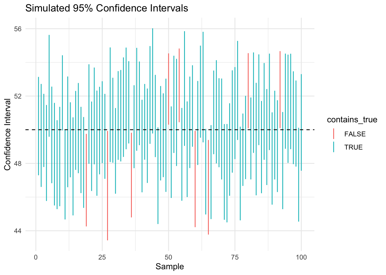
Visualizing Uncertainty

library(tidyverse)

Warning: package 'dplyr' was built under R version 4.5.1

── Attaching core tidyverse packages ──────────────────────── tidyverse 2.0.0 ──
✔ dplyr     1.2.0     ✔ readr     2.1.5
✔ forcats   1.0.0     ✔ stringr   1.5.1
✔ ggplot2   3.5.2     ✔ tibble    3.2.1
✔ lubridate 1.9.4     ✔ tidyr     1.3.1
✔ purrr     1.0.4     
── Conflicts ────────────────────────────────────────── tidyverse_conflicts() ──
✖ dplyr::filter() masks stats::filter()
✖ dplyr::lag()    masks stats::lag()
ℹ Use the conflicted package (<http://conflicted.r-lib.org/>) to force all conflicts to become errors

set.seed(123)

# Simulate many confidence intervals
true_mean <- 50
population <- rnorm(10000, mean = true_mean, sd = 10)

ci_sim <- replicate(100, {
  samp <- sample(population, 50)
  m <- mean(samp)
  se <- sd(samp)/sqrt(50)
  lower <- m - 1.96 * se
  upper <- m + 1.96 * se
  c(lower, upper)
})

ci_df <- as.data.frame(t(ci_sim))
names(ci_df) <- c("lower", "upper")
ci_df$id <- 1:nrow(ci_df)
ci_df$contains_true <- ci_df$lower <= true_mean & ci_df$upper >= true_mean

head(ci_df)

     lower    upper id contains_true
1 47.29454 53.13681  1          TRUE
2 46.60280 52.71860  2          TRUE
3 47.78533 52.12986  3          TRUE
4 45.76855 51.46971  4          TRUE
5 49.58307 55.63141  5          TRUE
6 46.82376 52.55915  6          TRUE

---

Plotting Confidence Intervals

ggplot(ci_df, aes(x = id, ymin = lower, ymax = upper, color = contains_true)) +
  geom_linerange() +
  geom_hline(yintercept = true_mean, linetype = "dashed") +
  labs(
    title = "Simulated 95% Confidence Intervals",
    x = "Sample",
    y = "Confidence Interval"
  ) +
  theme_minimal()

---

Key Insight

• Most intervals contain the true mean
  
• Some do not (about 5% for a 95% CI)

This is the meaning of “95% confidence”

---

Correct Interpretation

A correct interpretation is:

We are 95% confident that the true population parameter lies within this interval.

---

What “95% Confidence” Really Means

If we repeated the sampling process many times:

• 95% of constructed intervals would contain the true parameter
  
• 5% would miss it

---

Common Incorrect Interpretations

• ❌ “There is a 95% probability the true value is in this interval”
• ❌ “95% of individuals fall within this range”
• ❌ “The parameter changes from sample to sample”

---

Interpreting Instead of Calculating

In practice, you will often be given confidence intervals rather than calculating them.

Example:

Odds Ratio = 1.5 (95% CI: 1.2 to 1.9)

Interpretation:

• The exposure is associated with higher odds of the outcome
  
• The interval does not include 1 → statistically significant
  
• The plausible effect size ranges from 1.2 to 1.9

---

Width of Confidence Intervals

The width of a confidence interval depends on:

• Sample size (larger → narrower)
  
• Variability (higher → wider)
  
• Confidence level (higher → wider)

---

Demonstration: Sample Size Effect

set.seed(456)

get_ci_width <- function(n) {
  samp <- sample(population, n)
  se <- sd(samp)/sqrt(n)
  width <- (1.96 * se) * 2
  width
}

tibble(
  sample_size = c(50, 200, 500),
  ci_width = c(get_ci_width(50), get_ci_width(200), get_ci_width(500))
)

# A tibble: 3 × 2
  sample_size ci_width
        <dbl>    <dbl>
1          50     5.99
2         200     2.81
3         500     1.83

---

Communicating Uncertainty

In public health, it is essential to communicate uncertainty clearly.

Instead of saying:

“The intervention works”

Say:

“The intervention is associated with improved outcomes (95% CI: X to Y), suggesting a likely positive effect, though uncertainty remains.”

---

Public Health Example

Suppose:

• Screening rate = 72%
  
• 95% CI = 68% to 76%

Interpretation:

• The true screening rate is likely between 68% and 76%
  
• The estimate is reasonably precise
  
• Policy decisions should consider this range

---

Confidence Intervals & Hypothesis Testing

Confidence intervals are closely related to hypothesis testing.

Key connection:

• If the CI excludes the null value → statistically significant
  
• If the CI includes the null value → not statistically significant

Examples:

Measure	Null Value
Mean Difference	0
Risk Difference	0
Odds Ratio	1
Risk Ratio	1

---

Example Interpretation

If:

• Risk Ratio = 1.3 (95% CI: 0.9 to 1.8)

Then:

• CI includes 1 → not statistically significant
  
• Evidence is inconclusive

---

Key Terms

Term	Definition
Confidence Interval	Range of plausible values
Margin of Error	Distance from estimate to bounds
Precision	Narrowness of interval
Statistical Significance	CI excludes null value
Null Value	Value representing no effect

---

Practice Activity

1. Given a confidence interval, interpret it in plain language
   
2. Determine whether it is statistically significant
   
3. Identify whether the interval is wide or narrow
   
4. Explain what that implies about precision

---

Reflection Questions

1. Why are confidence intervals more informative than single estimates?
   
2. What does it mean when a confidence interval is wide?
   
3. How does sample size affect confidence intervals?
   
4. Why is correct interpretation important in public health?

---

Common Mistakes to Avoid

• Treating CI as probability of parameter
  
• Ignoring width of interval
  
• Overstating certainty
  
• Misinterpreting statistical significance

---

Conclusion

Confidence intervals provide a powerful way to communicate uncertainty.

They allow us to:

• quantify variability
  
• interpret results meaningfully
  
• connect estimation to decision-making

Understanding how to interpret and communicate confidence intervals is essential for evidence-based public health practice.

---

Looking Ahead

Next lesson:

• Hypothesis testing in depth
  
• p-values
  
• Type I and Type II errors
  
• Decision-making frameworks

---